Creating exponential buckets in QlikView™ charts

Despite the wide range of functionality QlikView™ is offering these days, I felt an exponential scale for creating buckets with the function CLASS would be a nice addition.
 
It took me some years to look into a solution for it, and yesterday I’ve finally decided it should be done. 😉
 
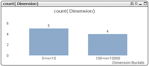
So here it is: instead of creating buckets with equally distanced boundaries, we can create now boundaries that can be defined as one or more powers of 10 (or anything else, of course).
 
To be more specific, you can, with this approach, to define boundaries like 1/10/100/1000/10000/etc or even like 1/1 k/1 mil/ etc
We used for all this, beyond CLASS function, some basic exponential and logarithmic equality and equivalency calculus.

As usually when trying to develop a certain new functionality or model, in QlikView™ or other software, I enjoy starting with a prototype that has a pretty simple set of data behind.

Some times I load this set of data using some short LOAD * INLINE , while in other occasions, when a data set with more cases is required, especially one that I am aware I will need to extend, I choose to have some Excel files/sheets as data sources.

In this case a single column of data and a single table with several rows would do the trick, so I used the INLINE approach:
 

LOAD * INLINE [
Dimension
1
2
30
40
50
600
700
800
900
];

As you can see, this data set has 2 values under 10, other 3 values under 100 and other 4 values under 1000

We’ve started with the regular approach: a calculated dimension CLASS (Dimension,BoundaryDistance) and a pretty simple function in the expression: count(Dimension) over a bar chart.

And this gave me a pretty easy to predict answer:

But this is a pretty ugly and kind of stupid visualization, right ?!
 
So, since we wanted an equally distanced boundary expressed in powers of 10, we changed first the formula to: CLASS (log10(Dimension),1) to see what happens:
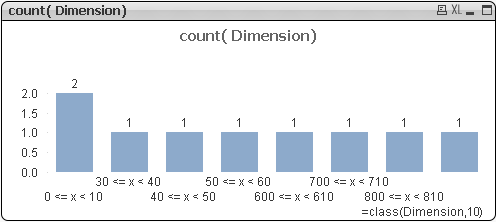
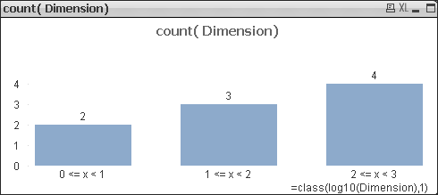
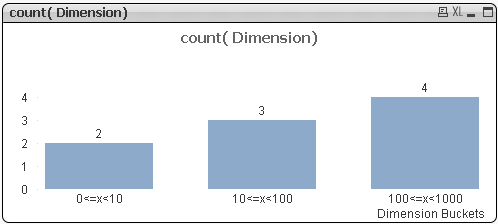
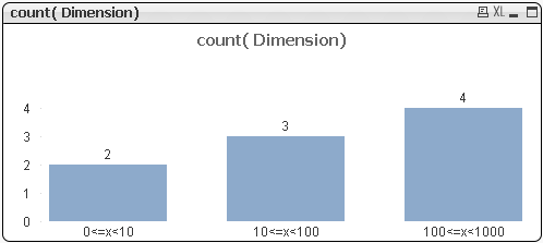
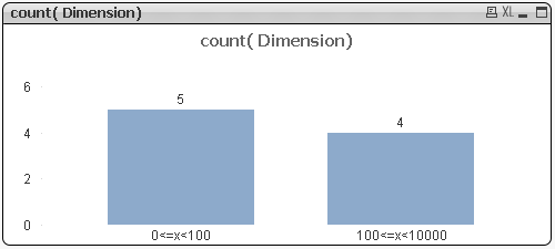
And the result , at least in terms of graphical representation, is already where I was dreaming to get.
 
Still, I wasn’t very happy with the labels and texts on the calculated dimension. My wish was to have texts on the dimensions closer to 0<=Dimension10<= Dimension
 
For this I felt I should dive into the DUAL functionality.
 
But trying to translate 10<=Dimension further, I’ve realized this is actually


where 1 and 2 has to be calculated first, for each interval, and afterwords calculate 10 raised at each of these exponents.
=> I’ve changed the calculated dimension to the following :

=dual(

pow(10,floor(log10(Dimension),1))

& ‘<=x<‘

& pow(10,ceil(log10(Dimension),1))

,class(log10(Dimension),1, ‘Dimension’)

)

(Used the FLOOR and CEIL functions within QlikView™ so that we can identify the next smaller and bigger integer for the logarithm).
 
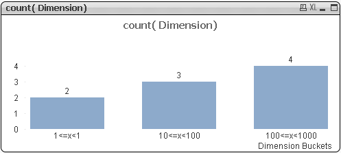
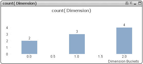
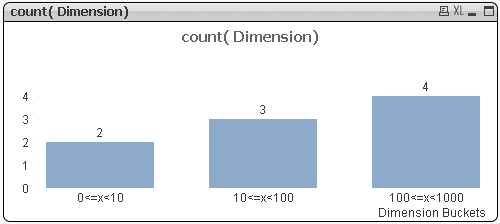
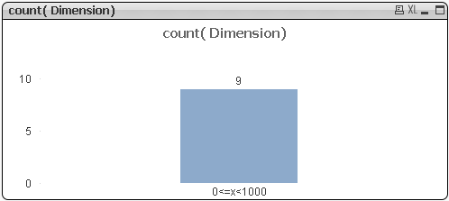
This DUAL approach is providing separate control on the numerical representation and the textual representation of the calculated dimension, and we have the following result:

All nice there with a small exception: the first interval seems pretty strange ! (1<=x)

At this moment I felt I should understand what numbers are actually behind each value within the calculated dimension, so I can better understand what is going on, and started to think about moving the numbers also in the text part of the DUAL function, perhaps using a NUM() function on top of the numerical part. But I remembered that a continuous dimension setting can do faster similar things for a CLASS calculated dimension.
 
So I’ve only checked the Continuous option within the Axes Properties Tab of the chart and got this.

Now, looking at the last 2 figures, it’s clear where the problem of the first bucket is coming from: we are attempting to use log(o) within the calculation steps of the first value within the calculated dimension.

But log(o) is minus infinite and therefore the calculation is going wild !

In order to solve also this last issue, I tried to use the higher boundary to identify the case and put the things in order. The next calculated dimension I’ve got is :

=dual(

if( pow(10,ceil(log10(Dimension),1))=1

, 0&'<=x<‘&10

,pow(10,floor(log10(Dimension),1))

&'<=x<‘

& pow(10,ceil(log10(Dimension),1))

)

,class(log10(Dimension),1)

)

and the new graphics (with Continuous Primary Dimension unchecked again) is looking like this:
This seems a pretty decent solution for interval boundaries on each power of ten.
 
Still we can go on further and add also the option to do from units to thousands and to millions, for instance.
 
For this I’ve introduced a variable, named Variable1, where I can keep the power of ten that we want to use for bucket wideness.
 
The new formula changed, under this circumstance to:

=dual(

if( pow(10,ceil(log10(Dimension),Variable1))=1

, 0&'<=x<‘&10

,pow(10,floor(log10(Dimension),Variable1))

&'<=x<‘

& pow(10,ceil(log10(Dimension),Variable1))

)

,class(log10(Dimension),Variable1 ))

and the graph is looking this way for Variable=1:

and like this for Variable=2:

We realize that again the first value is playing us some tricks here.
 
But, with some additional tweaking, the final formula I’ve made in this prototype is:
 
=dual(

if( pow(10,ceil(log10(Dimension),Variable1))=1

0&'<=x<‘& pow(10,Variable1) ,pow(10,floor(log10(Dimension),Variable1)) &'<=x<‘ &pow(10,ceil(log10(Dimension),Variable1))

) ,class(log10(Dimension),Variable1

))

and the results, for Variable1=1,2 and 3 are:
Final thoughts:
 
  • the calculated dimension option within QlikView™ is a pretty wild and powerful option, no doubt about it !
  • using small data prototypes to start from is always a wise idea !
  • try to “beautify” as much as possible your formulas and scripts ! (aka structure your code)
  • CEIL and FLOOR are so valuable !
  • saluting the LOG10() function. I kind of missed a LOG2() variation of this in some smart Gauge boundary limitations… (if anyone interested on this matter, let me know within a comment 😉